What is accuracy, precision, and bias?
Accuracy, precision, and bias represent the errors of the growth simulator, which are of different nature:
Precision represents the variation around average value. It stands for the so called random error (residual). Standard deviation is the precision measure.
Bias represents the constant (persistent) deviation from the real (target) value. It is a so called systematic error. Arithmetic average of the deviations from the real value is the measure of deviation.
Accuracy represents the variation around the real (target) value. It consists of the random error (residual) and of the systematic error (bias). Mean error is the measure of accuracy. If no systematic error exists, then accuracy is equal to precision. In such a case, the variation around the real value is equal to the variation around average value.
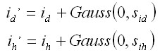
The principle is explained on an example of target-shooting (Figure 1).
|
Case A:
|
Average position of hits equals the value 10 (target centre). The variance of hits is small. |
|
Case B:
|
Average position of hits is not equal to the value 10 (target centre), but strongly deviates from it. The deviation is called bias. The variance of hits is small. |
|
Case C:
|
Average position of hits is equal to the value 10 (target centre). The variance of hits is large. |
|
Case D:
|
Average position of hits is not equal to the value 10 (target centre), but strongly deviates from it. The deviation is called bias. The variance of hits is large. |
Figure 1 Explanation of the terms accuracy, precision, and bias on an example of target shooting
How is empirical accuracy of the growth simulator examined?
Empirical accuracy of the growth simulator is examined using the repeated measurements of tree data from permanent plots. It is required that in subsequent periods the measurements of the variables are performed on the same trees (invisibly or visibly numbered) and that they are determined by the most precise method. From such data, real increments (ireal) of the variables are calculated. Starting from the initial situation in the plots, the simulation is run for the time period equal to the measurement interval, and modelled increments (imodel) of trees are derived. The plots with the most measured initial data that are required for the growth simulator (tree diameter and height, tree crown parameters, tree coordinates, climate and soil data) are preferred in order to keep the number of the generated initial characteristics at the lowest. The differences between the real and modelled tree increments are calculated, plotted against the modelled tree increments (Figure 2), and the regression analysis is performed. The calculated regression (red line in graph) represents the systematic error (bias), and the variation around the regression (green line in graph) represents the random error (residual).
Note: Modelled increment needs to be derived without any stochastic elements and mortality model has to be excluded from the simulation, because all live trees in the plots (inventory, monitoring, or research plots) are modelled.
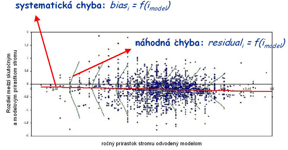
Figure 2 Principle of examining the empirical accuracy of the growth simulator
Although any suitable equation can be used in the regression analysis, straight line is the most common. Figure 3 presents a number of situations that can occur when the systematic error (bias) is derived:
| Case_A | Straight line and axis x are identical. The model does not have a systematic error: bias = 0 |
| Case_B | Straight line is parallel to axis x, and crosses the positive part of the axis y in the average value y. The model systematically underestimates the reality by the constant value regardless of the magnitude of the modelled increment: bias = y |
| Case_C | Straight line is parallel to axis x, and crosses the negative part of the axis y in the average value y. The model systematically overestimates the reality by the constant value regardless of the magnitude of the modelled increment: bias = y |
| Case_D | Straight line and axis x form a non-zero angle. The model has a systematic error of a varying magnitude which depends on the value of the modelled increment: biasi = f(imodel) |
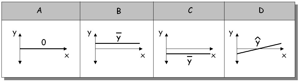
Figure 3 Different variants of the derivation of the model systematic error
When deriving the systematic error in the cases B, C, and D, a statistical test has to be performed to testify the error, since it could occur in the data under the influence of random factors resulting from the sampling. In the cases B and C, the significance test of the deviation of the arithmetic mean from zero is usually applied, while in the case D the significance test of the deviation of the correlation coefficient from zero, or the test of the deviation of absolute and regression coefficients from zero are performed (see relevant biometrical literature).
Random error (residual) is derived by a different method depending on the nature of values fluctuation around the regression. Here, two cases are possible (Figure 4):
| homoscedasticity | The variance of values around the regression line
is uniform.
|
| heteroscedasticity | The variance of values changes along the regression line. The regression relationship between the modelled increment and the random error: residuali = f(imodel) is used as a random error. |
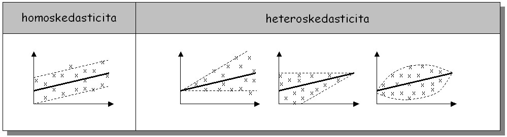
Figure 4 Different variants of the derivation of the model random error
The final empirical accuracy of the growth simulator is calculated as follows:
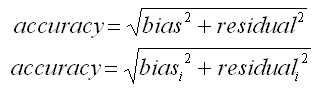
with regard to the fact, if systematic and random errors are constant (first formula), or variable depending on the value of the modelled increment (second formula). It is a mean model error, and represents the error span which can be reached with 68% probability. It means that if the simulation was repeated 100 times, in 68 cases the final value would differ from the reality by the mean error at maximum, while in the remaining 32 cases the real error would be greater. If we want to determine the error range with 95% probability, mean error has to be doubled (multiplied by 2).
What does the calibration of a growth simulator mean?
The calibration of a growth simulator means fitting the model to reality by error (accuracy) reproduction. The accuracy of the simulation is derived from the procedure described above. The reproduced error is randomly generated from Gauss distribution, which is defined by its arithmetical mean (bias) and its standard deviation (residual). The reproduced error is added to the modelled increment using one of the following equations:
ifinal = imodel + Gauss(bias,residual)
ifinal = imodel + Gauss(biasi,residuali)
with regard to the fact, if systematic and random errors are constant (first formula), or variable depending on the value of the modelled increment (second formula).
How is the growth simulator SIBYLA calibrated ?
|
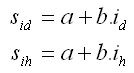
The growth simulator SIBYLA was calibrated using the repeated measurements of Slovak permanent monitoring plots. Height (ih') and diameter (id') increments of spruce, fir, pine, beech, and oak were calibrated. The systematic error (bias) of the model was not statistically proved. The random error was determined from the following regressions:
The final increment is then stochastically generated from Gauss curve as follows:
The coefficients of the regression (a, b) are published in Fabrika (2005). |
How is the theoretical precision of the growth simulator SIBYLA quantified ?
The growth simulator SIBYLA has stochastic nature. It means that slightly different results are obtained every time the simulation is repeated with the same initial conditions and settings. The source of the results randomness is the stochastic element in the modelling of tree height and diameter increment resulting from the calibration technique. However, the randomness is also caused by other reasons. In the growth simulator, the following components have stochastic nature:
calculation of tree diameter increment,
calculation of tree height increment,
generation of tree coordinates,
generation of tree quality,
determination of natural tree mortality,
determination of abrupt tree mortality caused by injurious agents.
Due to this, the theoretical model error can be calculated as a measure of the model precision. It suffices to repeat the simulation, to calculate the arithmetical mean of the analysed variable (e.g. volume), and then to calculate the theoretical mean error:
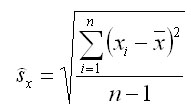
where xi are the results of the variable from repeated simulations, n is the number of simulations, and x is the arithmetical mean of the variable x. This mean error is the error of the variable x obtained from every simulation (i=1..n) with 68% probability, i.e. it represents the error if the simulation in such a forest stand, in such conditions, and settings was performed only once. The final simulation error of repeated simulations and for a pre-defined probability level is then calculated as follows:
sú odlišné výsledky veličiny z opakovaných simulácií, n je počet simulácií a x je aritmetický priemer veličiny x. Táto stredná chyba vyjadruje chybu veličiny x z každej jednej simulácie (i=1..n) so 68%-nou pravdepodobnosťou, to znamená chybu ak by sme simuláciu v podobnom poraste, podmienkach a nastaveniach urobili iba raz. Výsledná chyba simulácie pri opakovanom prevedení a pri vopred stanovenej pravdepodobnosti sa potom vypočíta podľa:
where t is the critical value of Student t-distribution (for 95% probability approx. 2.00). If the performed simulations are of higher importance and are to serve the practice, we suggest to repeat the simulations for the same initial conditions and settings 36 times at the minimum. It is optimal to repeat the generation of the structure 6 times, and to repeat the prognosis 6 times (in total 36 repetitions). Hence, the final value is equal to the arithmetical mean of the variable from the repeated measurements x. The final mean error of this average value is then 6 times lower than the mean error of a single simulation.
Unlike for yield tables, in the case of the growth simulator it is not possible to determine the mean simulation error that could be used generally, since the mean error depends on many factors. The following factors are considered to be the most important:
data source used for the structure generation,
complexity of the generated structure,
length of the period,
application of the disturbance model,
final characteristics from the simulation.
If permanent inventory plots with known tree information are taken as a data source, the mean error of the simulation will be lower than from less exact data, e.g. from summary stand data, data from yield tables, or description of selection forest. Similarly, the mean simulation error will be lower in even-aged, homogeneous stands with a simple stand structure than in the stands with a more complex structure, e.g. mixed, multi-storied, or uneven-aged stands, or selection forests. The mean error is also growing when the growth simulation is prolonged. In addition, the simulation accuracy is decreased when the disturbance model is activated. Even the final characteristic which is of our interest effects the mean simulation error. The error of an individual tree characteristic is much larger than the error of a mean or a summary stand characteristic. From stand characteristics, mean height and mean diameter have the lowest error. The error of the aggregated variable is larger, e.g. the error of mean stem volume, but this is still smaller than the error of stand volume per hectare, since this error contains also the error from tree number resulting from the stochastic mortality model.
Informatively, we determined the mean error of stand volume per hectare from 50-year simulation with excluded disturbance model. Mean errors of individual simulation are given below:
| simulation type | mean error (68% probability) | error at 95% probability |
| even-aged homogeneous stand generated from permanent research plots with known tree coordinates and tree characteristics | ±2,5% | ±5% |
| diversified stand with multiple stories generated from stand data | ±7,5% | ±15% |
| selection forest generated from forest description | ±15% | ±30% |
For the second type of the stand (i.e. diversified with multiple stories generated from stand data), mean errors of mean diameter and mean height were also determined: the errors of mean diameter were ±4% (with 68% probability), and ±8% (with 95% probability); the errors of mean height were ±3% (with 68% probability), and ±6% (with 95% probability).
How does the growth simulator SIBYLA coincide with yield tables?
Yield tables are considered a standard for the production of even-aged homogeneous stands. Therefore, the growth simulator can also be validated by comparing its output with yield tables under the same initial conditions. Although the growth simulator is capable of simulating a much wider range of stand structures than yield tables, it should be able to predict a similar development of even-aged homogeneous stands as yield tables. Hence, the growth simulator SIBYLA was verified also in this way. The procedure is described below:
Initial stands of spruce, fir, pine, beech, and oak aged 30 were generated for the lowest, medium, and the highest volume level, while the generation was initiated from the stand description of yield tables. The generation of the structure was repeated 6 times.
Detailed characteristics of air, climate, and soil were set to such values, that the development of the stand top height coincided with the development of the top height of a particular site class in yield tables.
Thinning regime was set to copy the thinnings in yield tables, i.e. 5-year period of thinnings was defined, and a neutral thinning with the intensity copying the development of the main crop volume in yield tables was selected.
The growth simulation was performed with the activated mortality model, with the stochastic element, and the correction of the edge effect, and without the disturbance model. The growth simulation was run for the period of 100 years, and repeated 6 times.
Average values of the volume development of the dominant and main crop were calculated from 36 simulations (6 structures x 6 prognoses). These values and the values from yield tables were plotted in graphs, and compared together.
The volume development in the growth simulator SIBYLA corresponds well with the development and in yield tables (Halaj et al. 1987) for all tree species and all site classes. However, the same trend was observed in almost all cases. For approximatelly 40 years, the development of volume is almost exact. Later on, SIBYLA produces slightly higher total current increments. This trend is visible in Figures 5 and 6 presenting the examples for spruce and beech and medium site classes. Nevertheless, the difference is not very distinct, and hence, we can state that the growth simulator SIBYLA is able to simulate forest stand development equally as yield tables, and can replace yield tables in even-aged homogeneous stands.
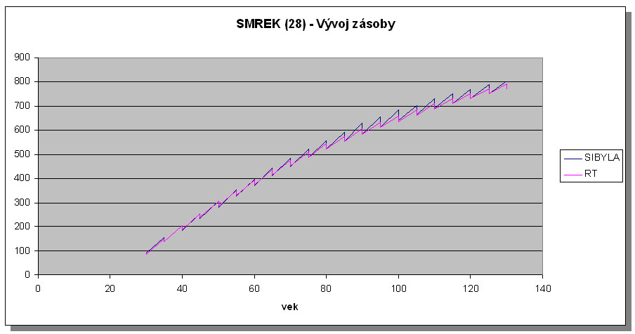
Figure 5 Comparison of the volume development of spruce in the site class 28 in the growth simulator SIBYLA and Slovak yield tables
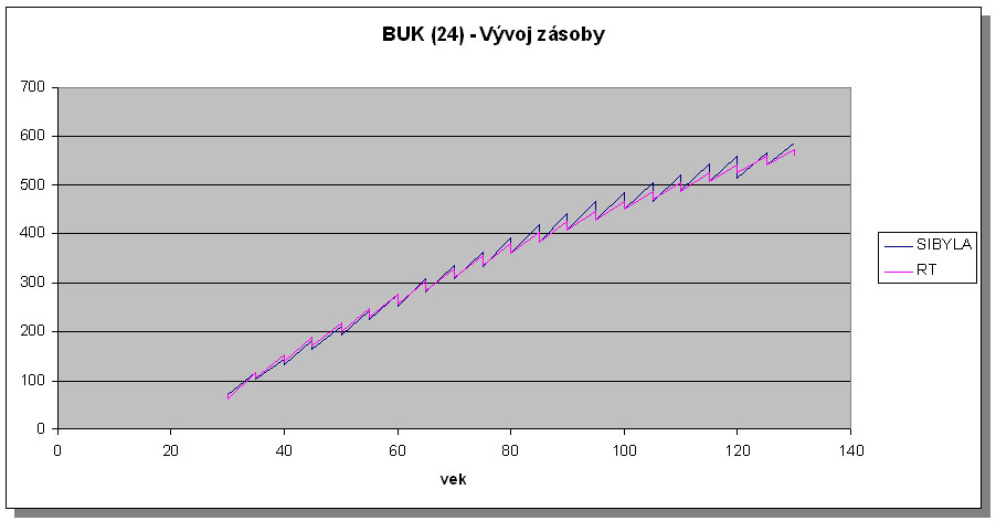
Figure 6 Comparison of the volume development of beech in the site class 24 in the growth simulator SIBYLA and Slovak yield tables
© Copyright doc. Ing. Marek Fabrika, PhD.
© Translated by Dr. Ing. Katarína Merganičová - FORIM