|
The algorithm that determines the
amount of trees to be removed or to be supported differs depending on the
treatment variant. The model offers the following variants:
A.
Thinning percentage
Thinning percentage represents the
relative amount of felled volume in per cents. It can be either static,
i.e. given for a particular simulation period, or dynamic, i.e.
modelled in relation to the value of the chosen growth variable x
(age, mean diameter, mean height, top height). In order to model dynamic
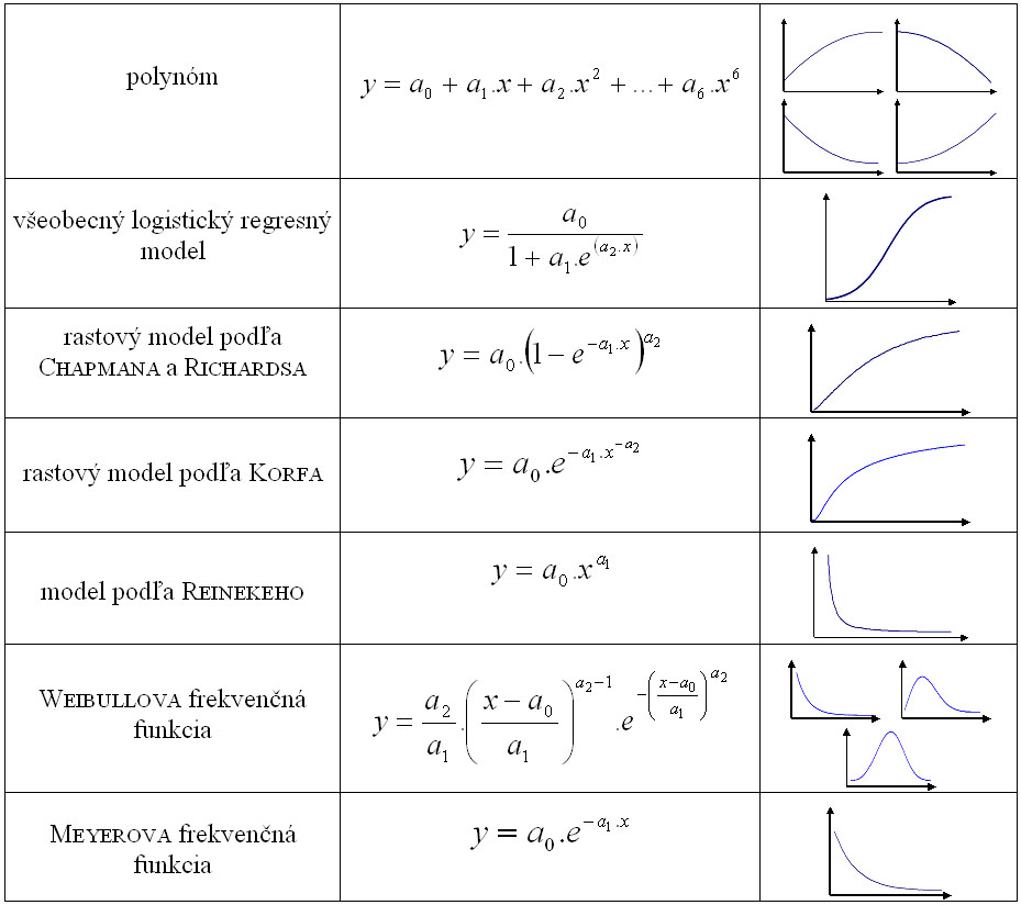
thinning percentage, a suitable function chosen from the model menu (Table 1) can be
utilised:
%VP = Additivity +
f(x) . Multiplier
where Additivity is a
constant
(by default 0), and Multiplier is an index (by default 1). The
additivity and multiplier move the function along
the axis y
in absolute or relative values according to the requirements.
The final volume of the secondary
crop is calculated from the initial volume of the dominant
crop as follows:
VP = VZ .
%VP : 100
By default, the growth simulator SIBYLA
applies the model of decennial thinning percentage of Halaj
et al. (1986), in which the percentage is related to stand age of all modelled
tree species, site classes, and degrees of stand density.
Table 1
Menu of mathematical functions
f(x) in SIBYLA
B.
Development curve of the main crop
The curve simulates the development
of a variable in the main crop
YH (volume, basal area, number of trees) related to the
value of the selected growth variable (age, mean diameter, mean height,
top height):
YH = f(x)
For the description of this
relationship, any function from Table 1 can be selected. The final amount of the
applied treatment is calculated on the
base of the initial value of the dominant crop YZ and
the area of the simulation plot in hectares (P) as follows:
YP = YZ -
[ Additivity + f(x) . Multiplier ] . P ; valid for YP
> 0
By default, the growth simulator SIBYLA
applies the model of the development of the main crop volume according to yield
tables (Halaj et
al. 1987), which depends on stand age of all modelled tree
species, site classes, and average stand volume level.
C. Stand density
of main crop
This parameter represents the
required relative degree of stand density. It can be either static,
i.e. given for a particular simulation period, or dynamic, i.e.
modelled in relation to the value of the chosen growth variable x
(age, mean diameter, mean height, top height). Dynamic stand density can
be modelled by a suitable function chosen from the model menu (Table 1):
SD = Additivity + f(x) .
Multiplier
The final volume of the secondary
crop is calculated from the initial volume of the dominant crop as follows:
VP = VZ -
SD . VH(RT) . (%R : 100) . P ; platí pre VP > 0
where VH(RT)
is volume of the main crop per hectare at full stand density and 100% tree
species composition derived from yield tables (Halaj
et al. 1987). By default, the growth simulator SIBYLA applies the
development of the tabular critical stand density according to Halaj
(1985) that is related to stand age separatelly for all
modelled tree species.
D.
Volume of secondary crop
This is the simplest variant
defined directly by the amount of volume to be felled in cubic metres in the
particular period, while the specified volume refers to the actual tree species
composition, actual stand density, and the size of the simulation
plot.
E.
Number of target (or promising) trees
As input, this model requires the number of future crop
trees
(NBRS
. ha-1). The reduction of
the number of trees on the area of the simulation plot is performed as
follows:
NBRS = (NBRS
. ha-1) . P
F.
Target distance between crop trees
This variant requires to specify
the theoretical
distance between future crop trees in metres (aBRS2).
The target number of trees in the simulation plot is calculated as:
NBRS = (10000 : aBRS2)
. P
G.
Clearing radius
It is necessary to specify the
radius of the circle around future crop trees in metres, in which no trees can exist. In this circle, all trees (except
for the future crop tree)
are felled regardless of their dimensions, competition pressure, quality,
or vitality degree.
H.
Degree of release
In this case, treatment intensity is specified by
the number of removed trees per one crop tree. Around each crop tree, a
pre-defined number of competitors is felled. In order to decide which trees are the
strongest competitors, the algorithm by Johann (1982)
is applied. The algorithm is based on the calculation of A-value for each potential
tree:
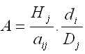
where aij is the
distance between the assessed future crop tree (j) and the
potential competitor (i), Hj is the height of the
future crop tree, Dj is the diameter of the future crop tree,
and di is the diameter of the potential competitor. The
greater the A-value, the higher the competition of the potential
competitor. The principle of the method is that the specified number of
the competitors with the highest
A-value is removed.
I.
Marginal distance
In this case, thinning intensity is
also based on the method of Johann (1982).
Unlike above, this variant requires the A-value to be determined, not the
number of trees. The marginal distance is calculated from the A-value, the diameter
and the height of the future crop tree, and the diameter of the potential competitor as
follows:
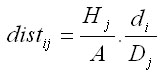
If the actual distance between the
crop tree and the potential competitor is lower than the marginal distance,
i.e. aij < distij
, the competitor is removed. Lower A-value indicates more
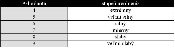
intense thinning. On the base of the A-value, Johann defined
different degrees of thinning intensity (Table 2), which are also applied
in the growth simulator SIBYLA.
J.
Target removal percentage
The principle of this variant is
that the percentual amount of trees (%dmax) with the diameter greater than or equal to dmax is felled. Hence,
the treatment intensity depends on the number of trees that reached or
exceeded the target diameter dmax and the percentage of
removed trees:
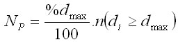
where n(di >= dmax)
is the number of trees with the diameter greater than or equal to the target
diameter.
K.
Removal curve
The removal curve assigns the
amount of removal to individual diameter classes on the base of the excess of the theoretical diameter frequency curve. Two variants are
provided:
1. GEOMETRICAL
DESCENDING SERIES of Liocurt.
The inputs of the model are the
rotation dimension (dmax) and the target
number of trees with the rotation dimension (nd max).
In the first step, an average quotient of the geometrical descending series is
determined as:
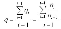
where nJ stands
for the number of trees of the particular tree species in ith
diameter class, while each diameter class is 4 cm wide, and the first diameter class
2 is in the range (0;4>. Extreme qi values,
i.e. the values below 1 and above 2 (inclusive), are excluded. For the
calculation of the theoretical frequency in diameter classes, the geometrical
descending series is used:
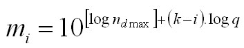
where mi is the
theoretical frequency of the particular tree species in ith
diameter class, and k
is the order of the diameter class, to which the tree with the rotation dimension belongs:
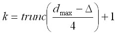
while delta is the accuracy
of the diameter dmax (=0.1 cm), and trunc is the
function for trimming the integral part of the result from the decimal
part. The number of trees removed from individual diameter classes
specifies a so
called removal curve, while the number is determined by comparing the actual tree species frequency in
the diameter class (ni)
with the modelled frequency (mi):
yi = ni -
mi ; platí pre yi > 0
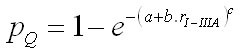
2. REGRESSION MODEL
OF FREQUENCY CURVE
In this variant, a theoretical
curve of frequency distribution is directly specified using the regression
model:
m = Additivity + f(d1.3) .
Multiplier
where m is the number of
trees with the diameter d1.3. Any function from Table 1 can
be applied (although Weibull and Meyer functions
are the most suitable). The resulting removal curve is calculated as:
yi = ni -
m(di) . h ; valid for yi > 0
where m(di) is
the number of trees derived from the model of frequency function for the
middle of ith diameter class and h is the width
of the diameter class (4 cm). By default, the growth simulator SIBYLA provides the
sample curves for selection forests of types A to E according to Meyer
(1952).
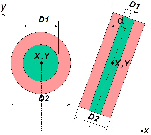
L. Size
of the cutting element
In this case, treatment intensity
is specified by the shape, size, and position of the cutting element. The
cutting element can take either the form of the so called patch cutting (circle)
or the form of strip cutting (strip). The circle is defined by the
coordinates of the central point (XOP
, YOP), as well as by inside and outside diameters (D1
, D2). The outside diameter D2 specifies
total patch size. The inside diameter D1 serves for the
protection of the inner part of the patch, and is used when the first
patch is enlarged for the next outer fringe area. If the whole stand
inside the patch is to be removed, the inside diameter D1
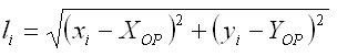
equals to 0. When applying this cutting type, the distance of each tree
characterised by coordinates xi
and yi from the central point of the patch is
calculated as follows:
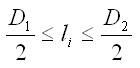
All trees having the diameter that
fulfils
the condition below are removed from the forest:
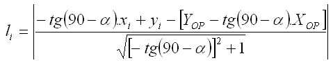
In the case of strip cutting, the
strip is defined by a point with coordinates XOP and YOP,
through which the central axis is running, by its inside and outside width
(D1 , D2), and by the azimuth measured
from the north, i.e. by the angle Alpha measured clockwise starting from
the positive axis y. The outside strip width represents the total
width of strip cutting. The inside width defines the central part of the
strip, which is kept away from felling. It is used when the original strip
is enlarged by next cutting elements outwards from the previous cutting.
When the whole strip width is to be cut, D1 is
equal to 0. The trees
are selected for cutting as follows. First, the perpendicular distance from the strip axis is
determined for each tree:
The tree is cut if its
perpendicular distance meets the condition below:
|