In the simulator, the following site variables are used:

• s₁ (N2O) ... NO_x concentration in air (ppb)

• s₂ (CO2) ... CO₂ concentration in air (ppm)

• s₃ (NUTR) ... soil nutrient supply (relative value in the range from 0 to 1)

• s₄ (DAYS) ... number of days in the vegetation period (days with daily mean temperature above 10°C)

• s₅ (TAMPL) ... annual temperature amplitude (the difference between annual minimum and maximum temperature in °C) 

• s₆ (TEMP) ... daily mean temperature in the vegetation period in °C (from April to September)

• s₇ (MOIST) ...soil moisture (relative value in the range from 0 to 1)

• s₈ (PRECIP) ... precipitation amount in the vegetation period in mm (from April to September)

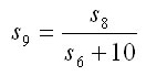
• s₉ (ARID)... aridity index according to de Martone in mm.°C^-1 derived as:

Transformation functions

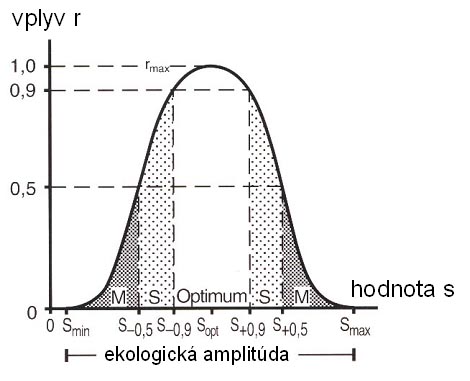
Transformation functions are used to transform the effect of site variables s_i to relative values. The functions are based on the theory of fuzzy sets. The principle is shown in Figure 1. On the axis x, the ecological amplitude of the characteristic s, i.e. its range from minimum to maximum value, in which the particular tree species can survive, is represented. The axis y depicts the transformed values of the influence r in the range from 0 to 1. The transformation function is simplified using the break points (c_j), between which the linearised transformation sections are formed as follows:  

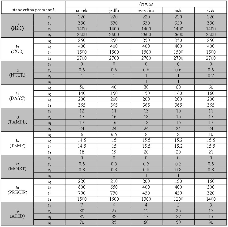
Table 1 presents the values of break points (c_j) for individual tree species.

Note: The growth simulator SIBYLA is parameterised only for spruce, fir, pine, beech, and oak. All other tree species are simulated on the base of the tree species with the closest production relationship !!! 

Table 1 Values of transformation function coefficients within the ecological amplitude (according to Kahn 1994)

Agregation functions

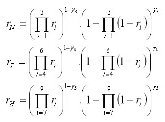
In the next step, total nutrition effect (r_N), total temperature effect (r_T), and total humidity effect (r_H) are calculated using the aggregation functions: 

Afterwards, the effects are aggregated to obtain three reduction factors: the reduction of the asymptote of the tree height growth potential (r_A), the reduction of the culmination age of the height increment potential (r_tkulm), and the reduction of the tree basal area increment potential (r_g) as follows:

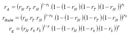
Gama coefficients are published in Fabrika (2005).

1. First, the coefficients A, k, p of Korf function applied for modelling the height growth potential are determined from the ecological site classification using the interpolation principle: 

A = A₀ + A₁ . r_A

t_kulm = t₀ + t₁ . r_tkulm

p = a₀ + a₁ . t_kulm + a₂ . t_kulm²

k = t_kulm^(p-1) . p

2. If the tree age is unknown, the theoretical age t is estimated from the growth potential using the actual tree height h:

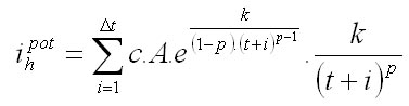
3. For the time period delta t = 1 year a potential tree height increment i_h^pot is calculated as follows:

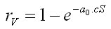
4. On the base of the tree crown lateral area cS, the reduction factor of tree vitality r_V is calculated as:

5. Using the characteristics obtained from the competition model, the reduction factor of the competition pressure on tree r_C is determined as: 

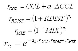
where delta CCL is the change of the competition index CCL  before and after the thinning treatment. The other competition characteristics represent the conditions after thinning. 

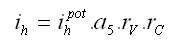
6. Finally, tree height increment i_h is calculated as follows:

7. and the residual element of the tree height increment, which includes the systematic error resulting from the model calibration, is generated: 

i_h' = i_h + Gauss(bias_ih, s_ih)

All coefficients were published in Fabrika (2005).

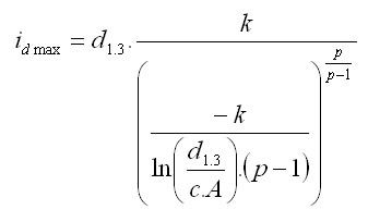
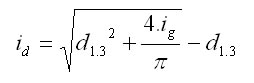
1.Using Korf function, maximum tree diameter increment i_dmax is calculated from the actual tree diameter:

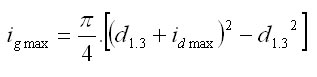
2. Maximum tree basal area increment i_gmax is determined from the actual (initial) tree diameter and the calculated maximum diameter increment using the mathematical relationship between the diameter and the basal area: 

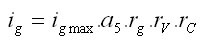
3. To obtain an expected tree basal area increment i_g, maximum basal area increment is reduced by the site reduction factor r_g, reduction factor of tree vitality r_V, and reduction factor of competition pressure r_C according to: 

4. Finally, the annual tree diameter increment is determined from the basal area increment using their mathematical relationship: 

5. At last, the residual element of the tree diameter increment, which also includes the systematic error resulting from the model calibration, is generated: 

i_d' = i_d + Gauss(bias_id, s_id)

All coefficients can be found in Fabrika (2005).

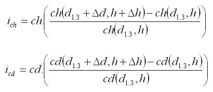
Crown parameters, i.e. height to crown base (ch) and crown diameter (cd), are derived indirectly using the so called cross relationships of the tree height and diameter increments. The increments of height to crown base (i_ch) and of crown diameter (i_cd) are then calculated as: 

Generation of climatic characteristics is based on climate regionalisation (Ďurský, Minďáš, Konôpka 2002), from which the table of climatic amplitudes was created (Borgoň 2003).

Climate regionalisation

The regionalisation of climate is based on the measurements from meteorological stations. For individual meteorological stations, necessary site variables (s₄,s₅,s₆,s₈) were calculated following the methodology of the World Meteorological Organisation (WMO). Regression equations describing the relationships between site variables and elevation of the weather station were derived: 

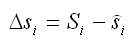
For each meteorological station the real error of the regression model was calculated as follows:

The errors were regionalised in GIS environment using spatial interpolation techniques. A raster layer of site variables was created on the base of the digital terrain model and the regression model. To this raster layer, the raster layer of the interpolated errors was added according to the rules of the map algebra: 

which resulted in corrected rasters of climatic site variables. The whole process is shown in Figure 2. 

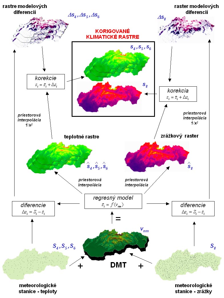
Figure 2 Regionalisation of climatic characteristics in GIS environment

Table of climatic amplitude(s)

For individual forest ecoregions of Slovakia, minimum (v_{nm min}) and maximum (v_{nm max}) elevations were derived, for which necessary site variables (,) were derived from climatic rasters. The results are saved in the database table. This table serves for the interpolation of site variables of the particular forest stand with regard to the forest ecoregion the stand belongs to, and its elevation (v_nm):  

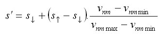
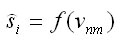
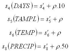
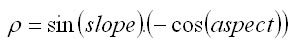
Finally, the interpolated site variable is adjusted by aspect and slope of the forest stand using the modifiers derived by Kahn (1994):

where

Site variables s₁ and s₂, i.e. the concentration of NO_x and CO₂ in air in ppb and ppm, respectively, are calculated from the regressions taken over from the model SILVA 2.2 (Kahn 1994). Their values depend on the calendar year (t):

s₁ = 287,6 + 0,00048 . (t - 1800)²

s₂ = 280,37 + 0,00177 . (t - 1800)²

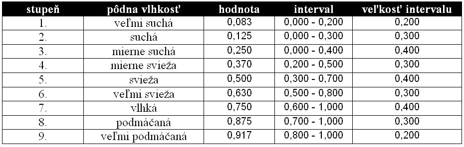
Soil site variables s₃ and s₇, i.e. soil nutrient supply and soil moisture, are transformed from the original relative values within the interval <0;1> to qualitative degrees with a predefined range of relative values and their mean as presented in Tables 2 and 3. For soil nutrient supply 5 degrees, and for soil moisture 9 degrees were distinguished. The degrees are adopted from Chen and Hwang (1992). The particular forest stand (simulation plot) is assigned the qualitative degree depending on the forest type the stand belongs to. Ujházy (2001) created the conversion table of forest types to degrees of soil moisture and soil nutrient supply. 

 Table 2 Values assigned to the degrees of soil nutrient supply 

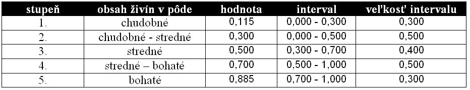
Table 3 Values assigned to the degrees of soil moisture